🙋FAQs (new)
Moving forward, we’re going to try and update this page each week to provide answers to questions asked (1) live in lecture, (2) at q.dsc40a.com during lecture, (3) on Campuswire, and (4) in the relevant Reflection and Feedback Form. If you have other related questions, feel free to post them on Campuswire.
Jump to:
- Week 9: Bayes’ theorem and Naive Bayes Classifier
- Week 7: Combinatorics
- Week 5: Gradient descent
- Week 4: Multiple linear regression
- Week 3: Linear Algebra
- Week 2: Loss Functions, and Simple Linear Regression
Week 9: Bayes’ Theorem and Naive Bayes Classifier
Why can we disregard the denominator in the Naive Bayes classifier?
In Naive Bayes, we want to compare the probability of a data point with given features belonging to different classes. The denominator, P(features), is the same for all classes and acts as a normalization factor. Since we’re only comparing relative probabilities, we can safely ignore this denominator without affecting the classification outcome.
Think of it like comparing fractions with the same denominator. The one with the larger numerator is the bigger fraction, even if we don’t know the exact denominator value. Similarly, in Naive Bayes, the class with the highest numerator P(features \(\vert\) class) * P(class) is the most likely class for the given data point.
Lecture(s) to Review:
Why do we divide by the marginal probability and not the prior probability in Bayes’ Theorem?
In Bayes’ theorem, we’re aiming to calculate the posterior probability, which is the probability of an event occurring after observing new evidence. The formula is:
\[P(A|B) = \frac{P(B|A) P(A)}{ P(B)}\]Let’s break down the components:
- \(P(A \vert B)\) Posterior probability - the probability of event A occurring given that event B has occurred.
- \(P(B \vert A)\) Likelihood - the probability of observing event B given that event A is true.
- \(P(A)\) Prior probability - the probability of event A occurring before observing any new evidence.
- \(P(B)\) Marginal probability (also called the evidence) - the probability of observing event B, regardless of whether A is true or false.
Why not divide by the prior, \(P(A)\)?
The prior probability, \(P(A)\), represents our initial belief about the likelihood of event A. While it’s important to consider our prior knowledge, it’s not sufficient for calculating the posterior probability. We need to account for the new evidence, B, which is captured by the likelihood, \(P(B\vert A)\).
Why divide by the marginal, \(P(B)\)?
The marginal probability, \(P(B)\), acts as a normalization factor. It ensures that the posterior probability, \(P(A\vert B)\), is a valid probability, meaning it sums to 1 across all possible values of A. By dividing by \(P(B)\), we’re adjusting the likelihood and prior to account for the overall probability of observing B.
In summary:
- The prior tells us our initial belief.
- The likelihood tells us how likely the evidence is given our belief.
- The marginal tells us how likely the evidence is overall.
- The posterior tells us how the belief has been updated given the evidence.
By combining these three elements using Bayes’ theorem, we can update our beliefs in light of new evidence.
Lecture(s) to Review:
Week 7 - Combinatorics
Permutations vs. Combinations
Permutations:
- Order matters The arrangement of items is important.
- Example Choosing a president, vice president, and treasurer from a group of 10 people. The order in which they are chosen matters.
- Formula: \(P(n,k) = \frac{n!} {(n-k)!}\)
Combinations:
- Order doesn’t matter The arrangement of items doesn’t matter.
- Example: Choosing 3 people from a group of 10 to form a committee. The order in which they are chosen doesn’t matter.
- Formula: \(C(n,k) = \frac{n!} {k! (n-k)!}\)
How to decide when to use permutations and when to use combinations?
Does the order matter?
- If yes: use permutations.
- If no: use combinations.
Example:
Let’s say you have 5 books and you want to choose 3 of them to read.
- If the order in which you read them matters (e.g., you want to read them in a specific sequence), you’d use permutations.
- If the order doesn’t matter (you just want to choose 3 books to read, regardless of the order), you’d use combinations.
Remember:
- Permutations overcount combinations.
- If you’re unsure, consider a smaller example and list out all the possibilities.
Lecture(s) to Review:
Why do we need to divide by the number of orderings when going from permutations to combinations?
When we transition from permutations to combinations, we’re essentially removing the significance of order. To illustrate this, let’s consider a simple example:
Imagine we have 3 letters: A, B, and C. We want to choose 2 of them.
If order matters, we have the following possibilities: AB, AC, BA, BC, CA, CB. Therefore there are 6 permutations.
If order doesn’t matter, we only care about the groups of 2 letters, not the specific order within each group. So, the following groups are considered the same:
- AB , BA
- AC , CA
- BC , CB
Each group of 2 letters has 2! (2 factorial) = 2 different orderings. To get the number of combinations, we need to divide the total number of permutations by the number of orderings for each group.
Combinations = Permutations / Number of Orderings per Group Combinations = 6 / 2 = 3
Generalizing the Concept: For any group of k items chosen from a set of n items, there are k! ways to arrange those k items. So, to get the number of combinations, we divide the number of permutations by k!:
Combinations = Permutations / k!
This division removes the impact of order, leaving us with the number of unique groups or combinations.
Lecture(s) to Review:
What is the difference between Sequences and Permutations?
Permutations are a specific form of Sequences in which we sample without replacement. For both sequences an permutations order matters (as opposed to sets and combinations). The main difference lies in the repetition of elements. In sequences, elements can be repeated, while in permutations, each element can only be used once.
Example:
- Sequences: Creating a 3-digit PIN code using digits 0-9. You can repeat digits, and the order matters (123 is different from 321).
- Permutations: Arranging 5 people in a line. Each person can only be in one position, and the order of the people matters.
Lecture(s) to Review:
Week 5: Gradient decent
In the formal definition of convexity, how did we obtain the expression for the line segment between \(f(a)\) and \(f(b)\)?
First we want to define a position \(x(t)\) on the \(x\) axis at time \(t\), where \(0 \leq t \leq 1\).
At time \(t=0\) we’re at \(a\), so \(x(0)=a\).
At time \(t=1\) we’re at \(b\), so \(x(1)=b\).
This formula satisifies these conditions:
\[x(t) = a + (b-a)t = a(1-t) + bt\]To obtain an expression for the line segment, recall a line is defined as
\[y(t) = w_1 t + w_0\]where \(w_1\) is the slope of the line and \(w_0\) is the intercept.
We have conditions: \(y(a)=y(x(t=0))=f(a)\) and \(y(b)=y(x(t=1))=f(b)\), so that the line segment intersects the function \(f(x)\) at \(a\) and \(b\).
Plug in \(t=0\):
\[y(a)=y(x(t=0))=w_1 \cdot 0 + w_0 = w_0 = f(a)\]Plug in \(t=1\)
\[y(b)=y(x(t=1))=w_1 \cdot 1 + w_0 = w_1+ w_0= w_1+ f(a)=f(b)\] \[w_1 = f(b)-f(a)\]Overall we get
\[y(t) = (f(b)-f(a))t+f(a)= f(a)(1-t)+f(b)t\]For the function, at any given point \(a \leq x(t) \leq b\):
\[f(x(t)) = f(a(1-t)+bt)\]And the convexity condition is then, that for any point \(a \leq x(t) \leq b\), the line segment needs to be above or equal to the function:
\[y(x(t)) \geq f(x(t))\] \[f(a)(1-t)+f(b)t \geq f(a(1-t)+bt)\]Lecture(s) to Review:
Week 4: Multiple linear regression
What’s the relationship between spans, projections, and multiple linear regression?
Spans
The span of a set of vectors \(\{\vec{x}_1, \vec{x}_2, \ldots, \vec{x}_d\}\) is the set of all possible linear combinations of these vectors. In other words, the span defines a subspace in \(\mathbb{R}^n\) that contains all possible combinations of the independent variables.
\[\text{Span}\{\vec{x}_1, \vec{x}_2, \ldots, \vec{x}_d\} = \{w_1 \vec{x}_1 + w_2 \vec{x}_2 + \ldots + w_d \vec{x}_d\}.\]In the context of multiple linear regression, the span of the feature vectors represents all possible values that can be predicted using a linear combination of the feature vectors.
Multiple Linear Regression
Tying this all together, one can frame multiple linear regression as a projection problem; Given some set of feature vectors \(\vec{x}_1, \vec{x}_2, ... , \vec{x}_d\), and an observation vector \(\vec{y}\), what are the scalars \(w_1, w_2, ... , w_p\) that give a vector in the span of the feature vectors that is the closest to \(\vec{y}\)?
In other words, how close can we get to the observed values of \(\vec{y}\), while in the span of our feature vectors?
This framing of multiple linear regression also leads us to the normal equations
\[\vec{w}^* = (X^\mathrm{T}X)^{-1}X^\mathrm{T}\vec{y}.\]For more visual intuition of this idea, check out this tutor-made animation!
Lecture(s) to Review:
Why does the design matrix have a column of all 1s?
In linear regression, the design matrix \(X\) represents the features \(x_1, x_2, \ldots, x_d\). Each row of \(X\) corresponds to one data point, and each column corresponds to one feature. The parameter vector \(\vec{w}\), which we multiply by \(X\) to obtain our predictions \(\vec{h}\), contains the weights for each feature, including the intercept or bias term \(w_0\).
The term \(w_0\) is a constant that helps adjust the linear regression model vertically. This term is universal between predictions. In other words, regardless of the values of the other features \(x_1, x_2, \ldots, x_d\), the value of \(w_0\) will be the same. Let’s explore how this relates to our design matrix.
When the design matrix \(X\) is multiplied by the parameter vector \(\mathbf{w}\), each row of \(X\) produces a prediction \(h\) depending on the values of the features in the row. Each value in the row is multiplied by its associated weight in the parameter vector, and the resulting products are summed to form a prediction. However, we want the weight associated with \(w_0\) to output the same constant bias term no matter the values in \(X\).
To ensure this, we include a column of 1s at the beginning of the design matrix \(X\). This column represents the constant contribution of the bias term \(w_0\), and will always be multiplied by \(w_0\) when a particular observation is being used to make a prediction. In other words, regardless of the values of the features in \(X\), every prediction will have \(w_0 \cdot 1\) added to it. Let’s give a quick example of this.
Suppose we have a linear regression problem with two features. The design matrix \(X\) is:
\[X = \begin{bmatrix} 1 & x_{11} & x_{12} \\ 1 & x_{21} & x_{22} \\ 1 & x_{31} & x_{32} \end{bmatrix}\]And the parameter vector \(\vec{w}\) is:
\[\vec{w} = \begin{bmatrix} w_0 \\ w_1 \\ w_2 \end{bmatrix}\]To obtain the predicted values \(\vec{h}\):
\[\vec{h} = X \vec{w} = \begin{bmatrix} 1 & x_{11} & x_{12} \\ 1 & x_{21} & x_{22} \\ 1 & x_{31} & x_{32} \end{bmatrix} \begin{bmatrix} w_0 \\ w_1 \\ w_2 \end{bmatrix} = \begin{bmatrix} w_0 + w_1 x_{11} + w_2 x_{12} \\ w_0 + w_1 x_{21} + w_2 x_{22} \\ w_0 + w_1 x_{31} + w_2 x_{32} \end{bmatrix}\]As you can see in this example, our predictions all included the constant bias term \(w_0\), because in forming our predictions, \(w_0\) was always scaled by \(1\), the first entry in each row of our design matrix. This setup ensures that the intercept is included in the model, and does not interfere with the relationship between the other features and the prediction.
Lecture(s) to Review:
In multiple linear regression, is \(\vec{h}^*\) orthogonal to \(\vec{y}\)?
\(\vec{h}^*\) is the optimal hypothesis vector; That is, \(\vec{h}^* = X\vec{w}^*\). This means that \(\vec{h}^*\) is the orthogonal projection of our observation vector \(\vec{y}\) into the span of our feature vectors \(\vec{x}^{(1)}, \vec{x}^{(2)}, ..., \vec{x}^{(d)}\). As such, \(\vec{h}^*\) is orthogonal to the error vector \(\vec{e} = \vec{y} - \vec{h}^*\). However, this relationship does not imply orthogonality with \(\vec{y}\), or any other vector aside from the error vector \(\vec{e}\)
Lecture(s) to Review:
Why does the multiple linear regression model with two features look like a plane?
When we perform multiple linear regression with two features, we take information from two independent variables and predict some value for our target variable. Let’s think about this relates to a plane, both algebraically and geometrically.
Algebraically, if our features are \(x_1\) and \(x_2\), our prediction function takes the form
\[H(\vec{x}) = w_0^* + w_1^*x_1 + w_2^*x_2,\]which is the general formula for a plane.
Geometrically, multiple linear regression with two features is the same idea:
Each feature (\(x_1\) and \(x_2\)) corresponds to one axis, and our target variable (the variable we are trying to predict), is represented by the vertical axis. When we vary the values on the \(x_1\) and \(x_2\) axes, we are exploring the values of our prediction function when we can vary \(2\) features- this forms a \(2\)-dimensional surface.
If this question also concerns why these predictions form a plane instead of some other surface, perhaps with curves or bends, we can also briefly address that. In a linear regression model, the relationship between the input features and the target variable is linear. This means that the predicted value is a linear combination of the input features, with each feature having a fixed weight (or coefficient). Another way to say this is that in a linear model with \(2\) feature vectors, our predictions must be within the span of our feature vectors. In \(3\) dimensions, this span is a plane (This concept is addressed in lectures 5 and 6, if you want a refresher on span!)
If we had a nonlinear prediction function with \(2\) features, we could see a prediction function that forms a curved surface in \(3\) dimensions. However, as a consequence of performing linear regression, our prediction function will form a plane.
For more visual intuition of this idea, check out the first 35 seconds of this video!
Lecture(s) to Review:
What is the projection of \(\vec{y}\) onto \(\text{span}(\vec{x})\) – is it \(w^*\) or \(w^* \vec{x}\)?
In multiple linear regression, the orthogonal projection of the vector \(\vec{y}\) onto the span of the vectors \(\{\vec{x}^{(1)}, \vec{x}^{(2)}, ..., \vec{x}^{(n)}\}\) is expressed as:
\[\vec{h}^* = X\vec{w}^*.\]Here, \(\vec{w}^*\) is a vector of scalar coefficients (\(w_1, w_2\), etc.), and \(X\) is the design matrix. In other words, \(\vec{w}^*\) provides the specific coefficients with which to form a linear combinations of your features to make predictions \(\vec{h}^*\).
So, to answer the question directly: \(w^* \vec{x}\) is the projection of \(\vec{y}\) onto \(\text{span}\{\vec{x}^{(1)}, \vec{x}^{(2)}, ..., \vec{x}^{(n)}\}\), and \(w^*\) is the set of scalars used to make this projection when multiplied with \(\vec{x}\)
Lecture(s) to Review:
Do the normal equations work even when there is only one column in the matrix \(X\)?
Yes! Let’s look at two different cases where this can occur.
Case 1: \(X\) is a column of ones
If \(X\) is a column of ones, the model \(H(\vec{x}) = w_0\) fits a constant line through the data. Using the normal equations,
\[\vec{1}^T \vec{1} w_0^* = \vec{1}^T \vec{y}.\]\(\vec{1}^T \vec{1} = n\), where \(n\) is the number of data points, and \(\vec{1}^T \mathbf{y} = \sum_{i=1}^n y_i\). Thus, the normal equations become:
\[n \cdot w_0^* = \sum_{i=1}^n y_i.\]And, solving for \(w_0^*\), we get
\[w_0^* = \frac{1}{n} \sum_{i=1}^n y_i,\]which is the mean of the target values.
Case 2: \(X\) has different values
Now, let’s imagine that \(X\) is a column vector with different values for each data point, representing a single feature:
\[X = \begin{bmatrix} x_1 \\ x_2 \\ \vdots \\ x_n \end{bmatrix}.\]In this case, the model \(H(x) = w_1^*x\) fits a line through the origin. The normal equations become
\[X^T X w_1^* = X^T \vec{y}.\]Calculating the elements, we have
\[\sum_{i=1}^n x_i^2 \cdot w_1^* = \sum_{i=1}^n x_i y_i,\]and the normal equations are reduced to
\[w_1^* = \frac{\sum_{i=1}^n x_i y_i}{\sum_{i=1}^n x_i^2}.\]So, to answer your question, we can absolutely use the normal equations when our design matrix \(X\) has only one column!
Lecture(s) to Review:
How to know if \(X^TX\) is invertible
\(X^TX\) is invertible if and only if the columns (features) of X are linearly independent.
Meaning: Linearly independence means no feature (column) can be written as a linear combination of others. Mathematically, if \(X\beta = 0\) implies \(\beta = 0\), then \(X^TX\) is invertible.
What it means if \(X^TX\) is not invertible
If \(X^TX\) is not invertible, it means: The features are linearly dependent, i.e., at least one column can be formed by combining others. This is called multicollinearity.
Consequences: 1, The Normal Equation \(w^* = (X^T X)^{-1} X^T y\) cannot be solved, because \((X^T X)^{-1}\) does not exist. 2, Multiple equally valid solutions for \(w^*\) exist (not unique).
When \(X^TX\) isn’t invertible, how do we solve the normal equations?
【This advanced material is NOT included in the scope of the course】
As a starting point, try researching the Moore-Penrose pseudo-inverse and ridge regression as two other approaches to solving for an optimal parameter vector!
The Moore–Penrose pseudoinverse, written as \(X^{+}\), is a generalization of the matrix inverse that works even when \(X^TX\) is not invertible.
Meaning:
1, The pseudoinverse provides a way to find a least-squares solution to the normal equations \(X^T X w = X^T y\), even if the columns of X are linearly dependent.
2, It chooses the solution \(w^*\) with the smallest possible length (minimum norm) among all valid solutions.
Formally, the solution is: \(w^* = X^{+} y\)
Why it works:
when \(X^{\mathsf T}X\) is invertible (full column rank):
\[X^{+} = (X^{\mathsf T}X)^{-1}X^{\mathsf T}, \qquad \hat{\vec{w}} = (X^{\mathsf T}X)^{-1}X^{\mathsf T}\vec{y}.\]When \(X^{\mathsf T}X\) is not invertible (rank-deficient or under/over-determined).
Define \(X^{+}\) via the SVD \(X = U\,\Sigma\,V^{\mathsf T}\):
\[X^{+} = V\,\Sigma^{+}\,U^{\mathsf T},\]where \(\Sigma^{+}\) is formed by taking reciprocals of the nonzero singular values in \(\Sigma\) and transposing the shape. This \(X^{+}\) is uniquely characterized by the Moore–Penrose conditions:
\[XX^{+}X = X, \qquad X^{+}XX^{+} = X^{+}, \qquad (XX^{+})^{\mathsf T} = XX^{+}, \qquad (X^{+}X)^{\mathsf T} = X^{+}X.\]These ensure a consistent least-squares solution even when \(X^{\mathsf T}X\) is singular.
Lecture(s) to Review:
What does \(X^T\)e = 0 mean in plain English?
X is the design matrix. It contains all features. Each column represents one feature.
e is residual vector. It represents the difference between predicted and actual value.
\(X^T\)e = 0 means that the dot product between each feature column in X (design matrix) and e equals 0.
The residuals are perpendicular (orthogonal) of all feature directions. This shows that the model’s predictions are already mathematically optimal. No further adjustment to the weights 𝑤 can make the error smaller.
1️, Define the residual:
\[e = y - Xw\]2️, Minimize the sum of squared errors:
\[R(w) = e^T e = (y - Xw)^T (y - Xw)\]3️, Take the derivative with respect to \(w\) and set it to 0 (condition for a minimum):
\[\frac{\partial R(w)}{\partial w} = -2X^T (y - Xw) = 0\]4️, Obtain the key conclusion:
\[X^T (y - Xw) = 0\]That is,
\[X^T e = 0\]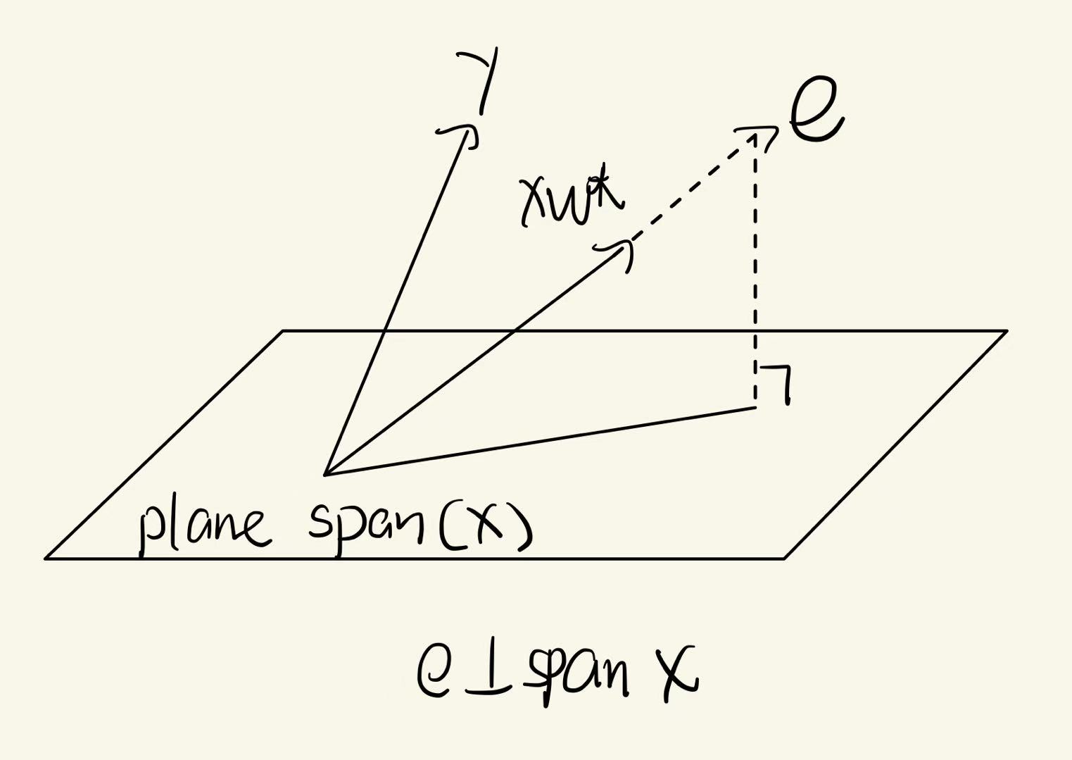
Week 3: Linear Algebra
How did we get from set of equations in \(w_1\) and \(w_2\) to the normal equations using orthogonality of the error vector?
Our objective was to find a more compact formulation of the following set of equations:
\(\vec{x}^{(1)} \cdot \vec{e} = 0\)
\(\vec{x}^{(2)} \cdot \vec{e} = 0\)
Denote the vector \(\vec{0}\) to be the vectors whose entries are all zero. Note that the set of equations can then be written in vector form as
\[\begin{bmatrix} \vec{x}^{(1)} \cdot \vec{e} \\ \vec{x}^{(2)} \cdot \vec{e} \end{bmatrix} = \begin{bmatrix} 0 \\ 0 \end{bmatrix} = \vec{0}\]The dot product \(\vec{a}\cdot \vec{b}\) can also be written as \(\vec{a}^T\vec{b}\), therefore:
\[\begin{bmatrix} \vec{x}^{(1)} \cdot \vec{e} \\ \vec{x}^{(2)} \cdot \vec{e} \end{bmatrix} = \begin{bmatrix} (\vec{x}^{(1)})^T \vec{e} \\ (\vec{x}^{(2)})^T \vec{e} \end{bmatrix}\]This vector can be written as the matrix-vector product of a matrix whose rows are the transpose of the column vectors \(\vec{x}^{(1)}, \vec{x}^{(2)}\) and the error vector \(\vec{e}\):
\[\begin{bmatrix} \text{ ----- } (\vec{x}^{(1)})^T \text{ ----- } \\ \text{ ----- } (\vec{x}^{(2)})^T \text{ ----- } \end{bmatrix} \vec{e} = \vec{0}\]The matrix whose rows are the transpose of the columns \(\vec{x}^{(1)}, \vec{x}^{(2)}\) is the matrix
\[X^T = \begin{bmatrix} \text{ ----- } (\vec{x}^{(1)})^T \text{ ----- } \\ \text{ ----- } (\vec{x}^{(2)})^T \text{ ----- } \end{bmatrix}\]Since we had earlier defined
\[X = \begin{bmatrix} \mid & \mid \\ \vec{x}^{(1)} & \vec{x}^{(2)} \\ \mid & \mid \\ \end{bmatrix}\]Thus we have simplified our set of equations to the form:
\[X^T \vec{e} =\vec{0}\]Finally we can plug in \(\vec{e} = \vec{y}-X\vec{w}\):
\[X^T \left(\vec{y}-X\vec{w}\right)=\vec{0}\]Lecture(s) to Review:
When do two vectors in \(\mathbb{R}^2\) span all of \(\mathbb{R}^2\)? When do \(n\) vectors in \(\mathbb{R}^n\) span all of \(\mathbb{R}^n\)?
Two vectors in \(\mathbb{R}^2\) span all of \(\mathbb{R}^2\) when they are linearly independent (You cannot express one as a scalar multiple of the other). In other words, if \(\vec{u}\) and \(\vec{v}\) are two vectors in \(\mathbb{R}^2\), they will span all of \(\mathbb{R}^2\) if \(\vec{u}\) and \(\vec{v}\) are not collinear, or on the same line.
Similarly, \(n\) vectors in \(\mathbb{R}^n\) span all of \(\mathbb{R}^n\) when they are linearly independent. This means that no vector in the set can be expressed as a linear combination of the others.
Intuition
To span a space means to cover it entirely.
Think of two vectors in \(\mathbb{R}^2\). If one vector is a scalar multiple of the other, then they both point in the same direction or opposite directions, essentially lying on the same line. This means they can only cover that line and cannot cover any other directions.
In higher dimensions, the same principle applies. For example, in \(\mathbb{R}^3\), three linearly independent vectors point in different directions and can cover all of three-dimensional space. However, if one is a linear combination of the others, then the three vectors lie on the same plane, and can only span that plane.
Lecture(s) to Review:
What is the projection of \(\vec{y}\) onto \(\text{span}(\vec{x})\) – is it \(w^*\) or \(w^* \vec{x}\)?
The orthogonal projection of the vector \(\vec{y}\) onto the span of the vectors \(\{\vec{x}^{(1)}, \vec{x}^{(2)}, ..., \vec{x}^{(n)}\}\) is expressed as:
\[X\vec{w}^*.\]Here, \(\vec{w}^*\) is a vector of scalar coefficients (\(w_1, w_2\), etc.), and \(X\) is the matrix whose columns are \(\{\vec{x}^{(1)}, \vec{x}^{(2)}, ..., \vec{x}^{(n)}\}\). In other words, \(\vec{w}^*\) provides the specific coefficients with which to form a linear combination of the vectors such that the resulting vectors is in the span and is as close as possible to \(\vec{y}\).
So, to answer the question directly: \(w^* \vec{x}\) is the projection of \(\vec{y}\) onto \(\text{span}\{\vec{x}^{(1)}, \vec{x}^{(2)}, ..., \vec{x}^{(n)}\}\), and \(w^*\) is the set of scalars used to make this projection when multiplied with \(\vec{x}\)
Lecture(s) to Review:
Do the normal equations work even when there is only one column in the matrix \(X\)?
Yes! Let’s look at two different cases where this can occur.
Case 1: \(X\) is a column of ones
If \(X\) is a column of ones, the model \(H(\vec{x}) = w_0\) fits a constant line through the data. Using the normal equations,
\[\vec{1}^T \vec{1} w_0^* = \vec{1}^T \vec{y}.\]\(\vec{1}^T \vec{1} = n\), where \(n\) is the number of data points, and \(\vec{1}^T \mathbf{y} = \sum_{i=1}^n y_i\). Thus, the normal equations become:
\[n \cdot w_0^* = \sum_{i=1}^n y_i.\]And, solving for \(w_0^*\), we get
\[w_0^* = \frac{1}{n} \sum_{i=1}^n y_i,\]which is the mean of the target values.
Case 2: \(X\) has different values
Now, let’s imagine that \(X\) is a column vector with different values for each data point, representing a single feature:
\[X = \begin{bmatrix} x_1 \\ x_2 \\ \vdots \\ x_n \end{bmatrix}.\]In this case, the model \(H(x) = w_1^*x\) fits a line through the origin. The normal equations become
\[X^T X w_1^* = X^T \vec{y}.\]Calculating the elements, we have
\[\sum_{i=1}^n x_i^2 \cdot w_1^* = \sum_{i=1}^n x_i y_i,\]and the normal equations are reduced to
\[w_1^* = \frac{\sum_{i=1}^n x_i y_i}{\sum_{i=1}^n x_i^2}.\]So, to answer your question, we can absolutely use the normal equations when our matrix \(X\) has only one column!
Lecture(s) to Review:
What does it mean for a matrix to be full rank?
A matrix is full rank when each column in the matrix is linearly independent.
In linear regression, the matrix \(X\) must be full rank to have a unique solution for the normal equations. If \(X\) is not full rank, it implies multicollinearity among the features, which leads to an infinite amount of solutions when solving for the optimal parameters \(\vec{w}^*\). For clarity:
Full Rank:
\[X^T X \vec{w}^* = X^T \vec{y}\]
If the matrix \(X\) is full rank, then all of its columns are linearly independent. This allows the normal equations:to have a unique solution.
Not Full Rank:
If \(X\) is not full rank, then some columns of \(X\) are linear combinations of other columns. This leads to multicollinearity, which results in infinitely many solutions for the normal equations.
Lecture(s) to Review:
What do you mean by “the inner dimensions need to match in order to perform matrix multiplication”?
Think about the multiplication of two matrices:
\[A = \begin{bmatrix} a_{11} & a_{12} & a_{13}\\ a_{21} & a_{22} & a_{23}\end{bmatrix} \text{ and } B = \begin{bmatrix} b_{11} & b_{12} \\ b_{21} & b_{22} \\ b_{31} & b_{32}\end{bmatrix}\]Let’s call \(C\) the product matrix between the two.
As we discussed in lecture, every entry of this resulting matrix \(C\) will be the result of the dot product of a row of \(A\) with a column of \(B\). For example, one entry of the product matrix \(C\) is formed by dotting \(\begin{bmatrix} a_{11} & a_{12} & a_{13}\end{bmatrix}\) with \(\begin{bmatrix}b_{11} \\ b_{21} \\ b_{31} \end{bmatrix}\).
This dot product is only possible if the “length” of each row in \(A\) is equal to the “height” of each column in \(B\). In our example, this dot product is defined by
\[\begin{bmatrix} (a_{11} \cdot b_{11}) + (a_{12} \cdot b_{21}) + (a_{13} \cdot b_{31}) \end{bmatrix}\]Clearly, if the number of entries in the first row of \(A\) were not equal to the number of entries in the first column of \(B\), this dot product would not make sense. For example, say \(B\) only had \(2\) rows. Then, when computing the entries of our product \(C\), we would run into a situation like this:
\[\begin{bmatrix} (a_{11} \cdot b_{11}) + (a_{12} \cdot b_{21}) + (a_{13} \cdot \text{...?}) \end{bmatrix}\]And we could not compute the entry of \(C\), making our matrix multiplication impossible.
In essence, the multiplication of matrices occurs when the inner dimensions of A and B, columns and rows, respectively, match. If they do not, the dot product between the rows of \(A\) and the columns of \(B\) would not be possible, and we cannot create a product matrix \(C\).
Lecture(s) to Review:
Is there a more detailed version of the MSE proof shown in Lecture 8?
Yes. Here’s a proof of the fact that \(R_\text{sq}(w_0^*, w_1^*) = \sigma_y^2 (1 - r^2)\).
First, note that since \(\sigma_x^2 = \frac{1}{n} \sum_{i=1}^n (x_i - \bar{x})^2\), we have that \(\sum_{i = 1}^n (x_i - \bar{x})^2 = n \sigma_x^2\). Then:
\(R_{\text{sq}}( w_0^*, w_1^* )\) = \(\frac{1}{n} \sum_{i=1}^{n} (y_i - \bar{y} - w_1^*(x_i - \bar{x}))^2\)
= \(\frac{1}{n} \sum_{i=1}^{n} \left[ (y_i - \bar{y})^2 - 2 w_1^*(x_i - \bar{x})(y_i - \bar{y}) + w_1^{*2} (x_i - \bar{x})^2 \right]\)
= \(\frac{1}{n} \sum_{i=1}^{n} (y_i - \bar{y})^2 - \frac{2w_1^*}{n} \sum_{i=1}^{n} ((x_i - \bar{x})(y_i - \bar{y})) + \frac{w_1^{*2}}{n} \sum_{i=1}^{n} (x_i - \bar{x})^2\)
= \(\sigma_y^2 - \frac{2w_1^*}{n} \sum_{i=1}^{n} ((x_i - \bar{x})(y_i - \bar{y})) + w_1^{*2} \sigma_x^2\)
= \(\sigma_y^2 - \frac{2w_1^*}{n} \frac{\sum_{i=1}^{n} ((x_i - \bar{x})(y_i - \bar{y}))}{\sum_{i=1}^{n} (x_i - \bar{x})^2} (\sum_{i=1}^{n} (x_i - \bar{x})^2) + r^2 \sigma_y^2\)
= \(\sigma_y^2 - 2w_1^* \frac{\sum_{i=1}^{n} ((x_i - \bar{x})(y_i - \bar{y}))}{\sum_{i=1}^{n} (x_i - \bar{x})^2} \frac{\sum_{i=1}^{n} (x_i - \bar{x})^2}{n} + r^2 \sigma_y^2\)
= \(\sigma_y^2 - 2w_1^{*2} \sigma_x^2 + r^2 \sigma_y^2\)
= \(\sigma_y^2 - 2(r^2\frac{\sigma_y^2}{\sigma_x^2}) \sigma_x^2 + r^2 \sigma_y^2\)
= \(\sigma_y^2 - 2r^2\sigma_y^2 + r^2 \sigma_y^2\)
= \(\sigma_y^2 - r^2 \sigma_y^2\)
= \(\sigma_y^2 (1 - r^2)\)
Lecture(s) to Review:
Week 1-2: Loss Functions and Simple Linear Regression
The Correct ERM (Empirical Risk Minimization) Modeling Steps
(1) Choose a model \(H(\mathbf{x}; \mathbf{w})\) — transform the abstract task into a concrete function class.
Without choosing the model first, you cannot properly define the parameters or the empirical risk.
(2) Choose a loss function \(L(y,\hat{y})\) — specify how prediction error is measured.
(3) Define the empirical risk \(R(\mathbf{w})\) — aggregate the loss over the dataset, e.g.
\(R(\mathbf{w})=\frac{1}{n}\sum_{i=1}^n L\big(y_i,\,H(\mathbf{x}_i;\mathbf{w})\big)\)
(4) Minimize \(R(\mathbf{w})\) — choose a solution method (closed-form, Gradient Descent, or other numerical optimization algorithms).
Common Misconceptions: Choose loss –> calculate risk –> take derivative –> set to zero This is the specific calculus-based solution for a specific model. If the loss function is non-differentiable, the model includes constraints, the optimization landscape is non-convex, or no closed-form solution exists, you should not use this approach. Instead, we must rely on more general optimization methods such as Gradient Descent (taught in week 5) or other numerical algorithms. In short, taking the derivative and setting it to zero is a method of solution, not a modeling step.
Isn’t the mean affected by outliers? How is it the best prediction?
A prediction is only the “best” relative to some loss function. When using the constant model, \(H(x) = h\), the mean is the best prediction only if we choose to use the squared loss function, \(L_\text{sq}(y_i, h) = (y_i - h)^2\). If we choose another loss function, like absolute loss \(L_\text{abs}(y_i, h) = \lvert y_i - h \rvert\), the mean is no longer the best prediction.
The key idea is that different loss functions lead to different “best” parameters.
Lecture(s) to Review:
Does Loss Function = Empirical Risk Function
Loss function \((y_i - \hat{y}_i)^2\): Error for a single data point Empirical risk function \(\frac{1}{n}\sum_{i=1}^n L(y_i, \hat{y}_i)\): The average of the loss over the entire dataset
Reminder: It is the empirical risk \(R(\mathbf{w})\) (which is a function of the model parameters \(\mathbf{w}\)) that we take the derivative of and minimize. Maintaining this distinction is vital for mathematical rigor as we move toward more complex models. You can find an exmaple for this concept below. The title is “Does empirical risk = mean squared error?”.
Does empirical risk = mean squared error?
“Empirical risk” is another term for “average loss for whatever loss function you’re using.” Any loss function \(L(y_i, h)\) can be used to create an empirical risk function \(R(h)\). We’ve seen two common loss function choices:
- When using absolute loss, \(L_\text{abs}(y_i, h) = \lvert y_i - h\rvert\), the empirical risk, \(R_\text{abs}(y_i, h) = \frac{1}{n} \sum_{i = 1}^n \lvert y_i - h\rvert\), has a special name: “mean absolute error.”
- When using squared loss, \(L_\text{sq}(y_i, h) = (y_i - h)^2\), the empirical risk, \(R_\text{sq}(y_i, h) = \frac{1}{n} \sum_{i = 1}^n (y_i - h)^2\), has a special name: “mean squared error.”
Lecture(s) to Review:
Why is MSE sensitive to outliers? (The Mathematical Mechanism)
The loss increases quadratically with the error. This mathematical mechanism causes large errors to contribute disproportionately more to the total loss. As a result, a few outliers can strongly influence the minimizer.
Example: If the prediction error is 10, the squared loss is 100. If the prediction error is 100, the squared loss jumps to 10,000. The error increased by 10×, but the loss increased by 100×.
Key Takeaway: MSE heavily penalizes large errors, making it highly sensitive to outliers.
Why is MAE robust to outliers?
The Mean Absolute Error (MAE) increases linearly with the prediction error. A large error and a small error affect the loss only in proportion to their magnitude, without the quadratic amplification seen in MSE. This means that a few extreme points will not overwhelmingly dominate the optimization process. As a result, MAE does not get “pulled” as strongly toward outliers, making it more robust to noisy or extreme observations.
Example: If the prediction error is 10, the loss contribution is 10. If the prediction error is 100, the loss contribution is 100. The loss increases by the same factor as the error.
Key Takeaway: MAE treats each data point’s error equally, so the optimization is driven by the entire dataset rather than just a few outliers.
The connection of MSE & MAE Minimizer and outliers
Minimizer Behavior: Minimizing MSE leads to the mean Minimizing MAE leads to the median
Why is the Mean sensitive to outliers? The mean tries to balance the squared errors. Because squaring amplifies large residuals, even a single extreme point contributes disproportionately to the total loss. Therefore, the mean will shift significantly toward the outlier to reduce the penalized error.
Why is the Median robust to outliers? The median depends only on the order of the data, not on the magnitude of deviations. Large errors and small errors influence the MAE only linearly, so a few extreme values cannot dominate the optimization. Thus, the median remains stable in the presence of outliers.
Key Takeaway: Squared Loss –> Mean –> Highly sensitive to outliers Absolute Loss –> Median –> Robust to outliers
What does it mean for a minimizer to be unique?
Let’s suppose we’re working with the constant model, \(H(x) = h\).
The minimizer of mean squared error is unique, because the minimizer of mean squared error for the constant model is the mean, and the mean of a collection of numbers \(y_1, y_2, ..., y_n\) is always just a single number. Specifically, it’s the number \(\frac{y_1 + y_2 + ... + y_n}{n}\).
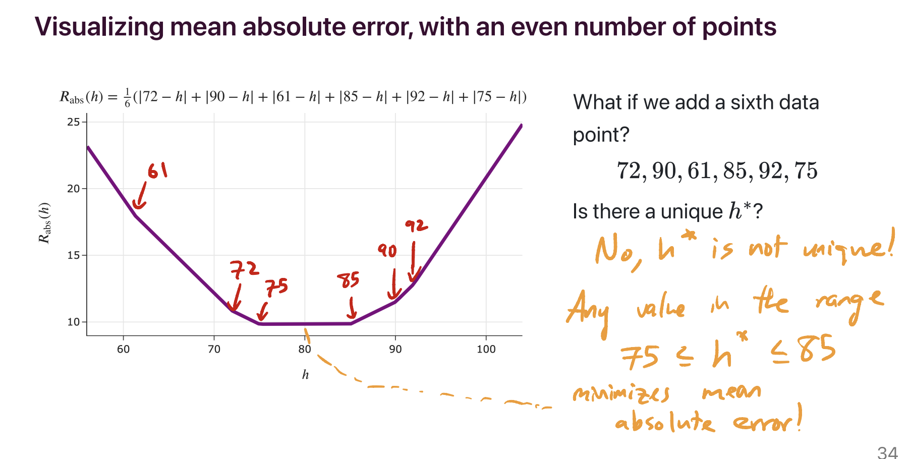
The minimizer of mean absolute error is not necessarily unique. It’s unique when there’s an odd number of data points – specifically, if the data points are sorted in order, with \(y_1\) being the smallest and \(y_n\) being the largest, then the minimizer of mean absolute error is the median, \(y_{\frac{n+1}{2}}\). But if there are an even number of data points, then any of the infinitely many numbers on the number line between \(y_{\frac{n}{2}}\) and \(y_{\frac{n}{2} + 1}\) minimize mean absolute error, so the minimizer of mean absolute error is not necessarily unique.
For example, in the dataset 72, 90, 61, 85, 92, 75, there are an infinite number of possible predictions that minimize mean absolute error. 75 is one of them, but so is 75.001, 76, 79.913, etc – anything between 75 and 85, inclusive, minimizes mean absolute error.
Lecture(s) to Review:
What was the point of plugging in \(h^*\) into \(R(h)\)?
We spent the first week of class minimizing empirical risk, \(R(h)\). We found that, depending on our choice of loss function, \(h^*\) ended up being a different measure of the center of our dataset. The point was to show that the values of \(R(h)\) actually have some meaning as well, and in particular, the smallest possible value of \(R(h)\) (which is \(R(h^*)\)) happens to describe the spread of our dataset.
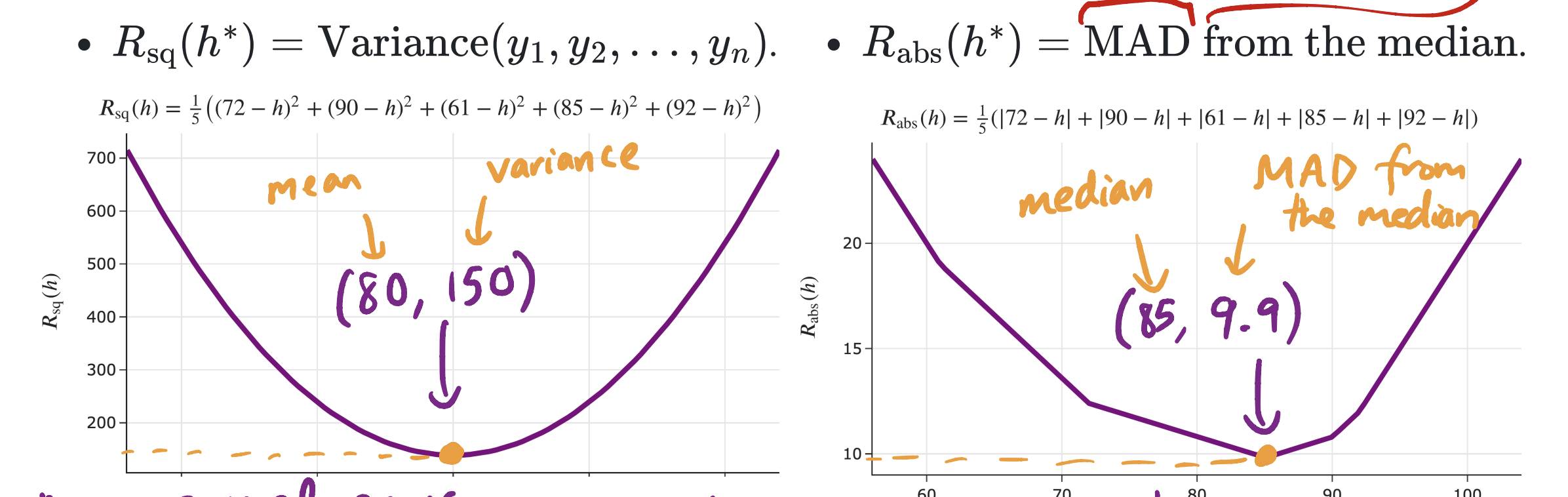
In the image above, \(h^*\) is the \(x\)-coordinate of the vertex (80 and 85). We know what 80 and 85 mean – they’re the mean and median of the dataset 72, 90, 61, 85, 92, respectively. What we were trying to give context to is what 150 and 9.9 mean – they’re the variance and the mean absolute deviation from the median of our dataset. Both the variance and mean absolute deviation from the median are measurements of spread.
Are there more loss functions outside of what we learned in class?
There are plenty! For example, there’s Huber loss, which is like a smoothed version of absolute loss (it’s absolute loss, with the corner at the bottom replaced with the bottom of a parabola). There’s also cross-entropy loss, also known as “log loss”, which is designed for models that predict probabilities (like logistic regression). These, and many more, will come up in future ML classes, like DSC 140A and CSE 158/DSC 148.
How do I know which loss function to choose in practice?
As we’ve seen, different loss functions have different properties. At least with regards to the constant model:
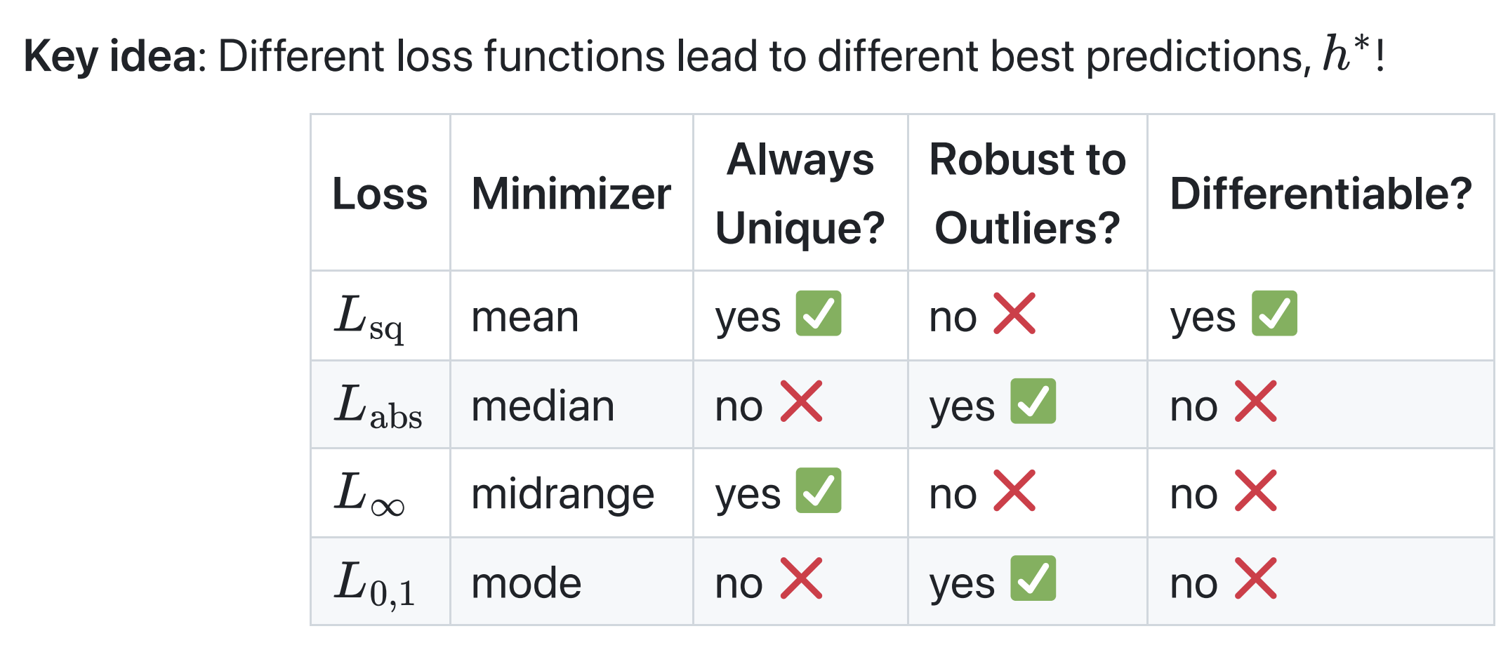
In practice, various models have a “default” choice of loss function. Regression usually uses squared loss, not just because squared loss is easily differentiable, but also because squared loss comes with lots of nice theoretical properties (which you’ll learn about in DSC 140A, like the fact that implicitly assumes that the distribution of errors is normal/Gaussian). But depending on your model, you can just try different loss functions and see which ends up creating the model with the best performance!
Lecture(s) to Review:
What was the point of the midrange and infinity loss? Will I actually use that in practice? (What is the infinity loss and why does the midrange minimize it?)
I’ve never heard of anyone using \(\lvert y_i - h\rvert^p\) with \(p \rightarrow \infty\) as a loss function in practice, so no. But the point of us studying that was for us to get a better understanding of how different loss functions penalize different kinds of errors, and in particular, how the optimal constant prediction is influenced by outliers.
Again, for the constant model \(H(x) = h\):
- Absolute loss, \(\lvert y_i - h\rvert\), isn’t sensitive to outliers, it’s very robust. Remember, the minimizer (the median) was found by finding the \(h\) where (# points to the left of \(h\) = # points to the right of \(h\)).
- Squared loss, \((y_i - h)^2\), is more sensitive to outliers. Remember, the minimizer (the mean) was found by finding the \(h\) where \(-\frac{2}{n} \sum_{i = 1}^n (y_i - h)= 0\), because \(-\frac{2}{n} \sum_{i = 1}^n (y_i - h)\) is the derivative of \(R_\text{sq}(h) = \frac{1}{n} \sum_{i = 1}^n (y_i - h)^2\). Since this is the case, the mean is “pulled” in the direction of the outliers, since it needs to balance the deviations.
- Following the pattern, \(\lvert y_i - h\rvert^3\) would be even more sensitive to outliers.
As we keep increasing the exponent, \(\lvert y_i - h\rvert^p\) creates a prediction that’s extremely sensitive to outliers, to the point where its goal is to balance the worst case (maximum distance) from any one point. That’s where the midrange comes in. It’s in the middle of the data, so it’s not too far from any one point.
why does the midrange minimize it? In short, its goal is to balance the worst case (maximum distance) from any one point. That’s where the midrange comes in. It’s in the middle of the data, so it’s not too far from any one point.
So while no, you won’t really use the idea of “infinity loss” in practice, I hope that by deeply understanding how it works, you’ll better understand how loss functions (including those we haven’t seen in class, but do exist in the real world) work and impact your predictions.
What does the limit \((p \to \infty)\) mean for the \(L_p \text{ norm}\)?
\(\Vert \mathbf{e} \Vert_p = \left( \sum_{i=1}^n |e_i|^p \right)^{1/p}\)
As (p) increases, large errors are penalized more heavily. Taking the limit: \(\lim_{p \to \infty} \Vert \mathbf{e} \Vert_p = \max_i |e_i|\)
So \((L_\infty)\) is the limit case of \(L_p \text{ norm}\).
Why do we use the \(L_p \text{ norm}\) to define the \(L_p \text{ loss}\)
Residuals form a vector of errors: \(\mathbf{e} = \mathbf{y} - \hat{\mathbf{y}}\)
We use the vector norm to define the loss: \(L_p(\mathbf{e}) = \Vert \mathbf{e} \Vert_p\)
Norms measure the magnitude of the error vector → this becomes the loss we minimize. Different \(p\) values give different robustness to outliers.
Lecture(s) to Review:
- Lecture 4 (Slide 19)
In Lecture 6, is the \(x_i\) not part of the summation since it is out of the parentheses?
The question was referring to a summation like this one:
\[\sum_{i = 1}^n (y_i - w_0 - w_1 x_i) x_i\]Here, \(x_i\) is indeed a part of the summation. The sum is of \(n\) terms, each of which are the form \((y_i - w_0 - w_1 x_i) \cdot x_i\). That is, the summation above is equivalent to:
\[\sum_{i = 1}^n \left( (y_i - w_0 - w_1 x_i) x_i \right)\]On the other hand, the following expression is invalid, since \(x_i\) doesn’t have any meaning when not part of a summation over \(i\):
\[\left( \sum_{i = 1}^n (y_i - w_0 - w_1 x_i) \right) x_i\]Lecture(s) to Review:
What was the 3D graph in Lecture 5 about?
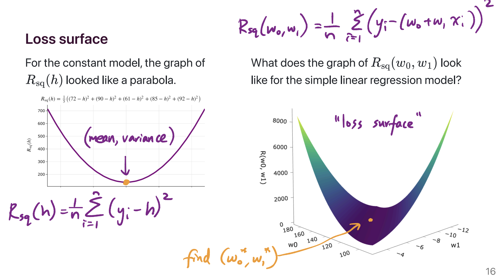
On the left, we have the graph of the mean squared error of a constant prediction, \(h\), on the dataset 72, 90, 61, 85, 92. It shows us that there is some best \(h\), which we’ve been calling \(h^*\), that makes the mean squared error as small as possible. We showed, using calculus, that the value of \(h^*\) for any dataset is \(\text{Mean}(y_1, y_2, ..., y_n)\).
On the right, we have the graph of mean squared error of the line \(H(x) = w_0 + w_1 x\). The dataset is the dataset of departure times and commute times we’ve been using as our running example. Specifically:
The two axes on the “ground” of the plot represent different intercepts, \(w_0\), and slopes, \(w_1\), that we could be using for making predictions.
The height of the graph above any \((w_0, w_1)\) pair is \(\frac{1}{n} \sum_{i = 1}^n (y_i - (w_0 + w_1 x_i))^2\). \(x_i\) represents the \(i\)th departure time (e.g. 8.5, corresponding to 8:30AM) and \(y_i\) represents the \(i\)th actual commute time (e.g. 75 minutes).
The point was to show what the function \(R_\text{sq}(w_0, w_1) = \frac{1}{n} \sum_{i = 1}^n (y_i - (w_0 + w_1 x_i))^2\) actually looks like, before we went to use calculus to minimize it. It kind of looks like a bowl, and has a clearly defined minimum. Calculus helped us find that minimum, which occurs at \(w_0^* = \bar{y} - w_1^* \bar{x}\) and \(w_1^* = \frac{\sum_{i = 1}^n (x_i - \bar{x})(y_i - \bar{y})}{\sum_{i = 1}^n (x_i - \bar{x})^2}\).
Lecture(s) to Review:
Can we minimize the mean absolute error of the simple linear regression model?
Yes, we can! The issue is just that there doesn’t exist a closed-form solution, i.e. a formula, for the optimal \(w_0^*\) and \(w_1^*\) in:
\[R_\text{abs}(w_0, w_1) = \frac{1}{n} \sum_{i = 1}^n \lvert y_i - (w_0 + w_1 x_i) \rvert\]So, we have to use the computer to approximate the answer. Regression with squared loss is called “least squares regression,” but regression with absolute loss is called “least absolute deviations regression.” You can learn more here!
Can you recap the proof of the formula for \(w_1^*\) that includes \(r\)?
Sure!
Let’s start with the formulas for \(w_1^*\) and \(r\):
\[w_1^* = \frac{\sum_{i=1}^n (x_i - \bar{x})(y_i - \bar{y})}{\sum_{i=1}^n (x_i - \bar{x})^2}\] \[r = \frac{1}{n} \sum_{i=1}^n \left(\frac{(x_i - \bar{x})}{\sigma_x}\right) \left(\frac{(y_i - \bar{y})}{\sigma_y}\right).\]Let’s try to rewrite the formula for \(w_1^*\) in terms of \(r\).
Step 1: Numerator
First, we can simplify the formula for \(r\) by factoring \(\sigma_x \sigma_y\) out of the summation.
\[r = \frac{1}{n \sigma_x \sigma_y} \sum_{i=1}^n (x_i - \bar{x})(y_i - \bar{y}).\]Rearranging this gives us the very pretty
\[\sum_{i=1}^n (x_i - \bar{x})(y_i - \bar{y}) = rn\sigma_x\sigma_y.\]Therefore, the numerator of the formula for \(w_1^*\) can be expressed as \(rn\sigma_x\sigma_y\).
Step 2: Denominator
Let’s start with the formula standard deviation \(\sigma_x\) defined as
\[\sigma_x = \sqrt{\frac{1}{n}\sum_{i=1}^n (x_i - \bar{x})^2}.\]This means that the variance \(\sigma_x^2\) is
\[\sigma_x^2 = \frac{1}{n}\sum_{i=1}^n (x_i - \bar{x})^2.\]Multiplying through by \(n\) gives
\[n\sigma_x^2 = \sum_{i=1}^n (x_i - \bar{x})^2.\]Therefore, the denominator of the formula for \(w_1^*\) can be expressed as \(n\sigma_x^2\).
Conclusion
Putting these parts together, we can rewrite the original formula for \(w_1^*\):
\[w_1^* = \frac{rn\sigma_x\sigma_y}{n\sigma_x^2}.\]And, simplifying this expression, we arrive at a beautiful result:
\[w_1^* = r \cdot \frac{\sigma_y}{\sigma_x}.\]Lecture(s) to Review
- Lecture 5 (Slide 18)
Is the correlation the same thing as the linear regression line?
No, they are different tools. Think of it this way:
- Correlation (\(r\)): This is like a report card that gives a single score (from -1 to 1) describing the potential for a straight-line relationship between two variables. It tells you how good of a relationship exists.
- Simple Linear Regression (SLR): This is the actual prediction tool (the line itself). It is the mechanism we use to draw the mathematically “best possible” straight line to capture that relationship.
If the correlation’s “report card” score is close to \(\pm 1\), it means the straight line (SLR) will be a very reliable and accurate prediction tool. If the correlation is close to 0, the SLR line is still the “best” straight line, but it will be a terrible, unreliable predictor.